Índice
Dev
Arduino line follower
DONE Arduino Zumo Siguelineas Evita obstaculos
Este proyecto forma parte de un trabajo para la asignatura Robótica Móvil y Neurobótica del Máster en Ciencia de Datos de la ETSIIT. Sus autores son Cristina Heredia y Alejandro Alcalde. El código está disponible en HerAlc/LineFollowerObstacles
El proyecto se compone de dos partes. La primera consiste en crear un robot que siga un camino pre-establecido marcado con líneas, además, debe evitar cualquier obstáculo que se encuentre en el camino. En caso de encontrarse con un obstáculo, el robot se detiene unos segundos y avisa, si pasado un tiempo el obstáculo sigue presente, el robot da media vuelta y sigue en camino contrario. La segunda parte se trata de implementar este funcionamiento en el entorno simulado Vrep.
Arduino
Para esta parte se ha implementado un Zumo capaz de conducir por sí mismo con las siguientes funcionalidades:
- Sigue Líneas
- Detección de obstáculos y toma de decisiones.
- Avisos sonoros a los obstáculos.
Para el sigue líneas se usan tres sensores sigue líneas para detectar cambios de intensidad.
Antes de comenzar, el robot necesita calibrar el giroscopio y los sensores sigue líneas. Para ello hay que pulsar el botón A una vez, esto calibra el giroscopio. Pulsar el botón A una segunda vez calibra los sensores sigue líneas.
Cabe mencionar que se parte del ejemplo Sigue Líneas de Arduino, disponible en el IDE de Arduino, las modificaciones realizadas han sido las siguientes:
Se integra código del ejemplo MazeSolver, que hace uso del giroscopio, en concreto los ficheros TurnSensor.h y TurnSensor.cpp. Esto permite calibrar el giroscopio, el cual es necesario para conseguir que el robot de media vuelta e inicie el camino contrario si el obstáculo que encuentra en su camino no se retira en tres segundos.
Para la detección de obstáculos se hace uso de un sensor de proximidad. La distancia a la que se para el robot se fija al valor 6. Cuando el robot se detiene al encontrar un obstáculo, avisa con una melodía simple compuesta por nosotros y similar al claxon de un vehículo. Finalmente, cuando el robot espera más de tres segundos y el obstáculo sigue presente, avisa con otra melodía compuesta por nosotros e inicia al camino en sentido opuesto girando 180 grados.
Vídeo
VREP
Para el proyecto en VREP se ha implementado un robot Sigue Líneas que se detiene ante la presencia de un obstáculo. Si el obstáculo se retira durante la simulación, el robot sigue su camino. Si el obstáculo no se retira, el robot permanece sin moverse para evitar chocar con él.
Para seguir las líneas se ha adaptado el ejemplo de VREP LineFollowerBubbleRob para hacerlo funcionar con Zumo, usando el modelo proporcionado en clase. La adaptación ha consistido en modificar el código de BubbleRob, que solo tiene dos motores, y hacerlo funcionar en el Zumo, con cuatro motores. Para ello se han tenido que ajustar parámetros de torque, peso etc de acuerdo al Zumo. También se desactivó el comportamiento cíclico de los motores.
Para evitar obstáculos se añade al robot un sensor de proximidad frontal, de forma similar al que se hizo en clase. Cuando el objeto se detecta a una distancia mínima pre-establecida, se detienen los motores del robot durante tres segundos. Transcurrido este tiempo, se vuelven a leer los datos del sensor de proximidad para comprobar si el objeto sigue presente o no. En caso de estar presente, el robot permanece parado, de lo contrario reanuda su marcha.
A continuación se muestra el código principal que controla el Zumo.
function sysCall_actuation()
    currTime = sim.getSimulationTime()
    result,distance=sim.readProximitySensor(noseSensor)

    if (result == 1 and distance < .25) then
        speed = 0
        if (objectDetected == false) then
            timeOjectDetected = sim.getSimulationTime()
            objectDetected = true
        end
        --sim.addStatusbarMessage(tostring(timeOjectDetected))
    end
    timeWaitingDetectedObject = currTime - timeOjectDetected
    sim.addStatusbarMessage(tostring(timeWaitingDetectedObject))
    -- After 3 seconds, check if continue foward or turn back
    if (timeWaitingDetectedObject > 3 ) then
        result,distance=sim.readProximitySensor(noseSensor)
        if (result == 0) then
            speed = -5
            timeOjectDetected = 0
            objectDetected = false
        end
    end

    -- read the line detection sensors:
    sensorReading={false,false,false}
    for i=1,3,1 do
        result,data=sim.readVisionSensor(floorSensorHandles[i])
        if (result>=0) then
            -- data[11] is the average of intensity of the image
            sensorReading[i]=(data[11]<0.3)
        end
    end

    rightV=speed
    leftV=speed

    if sensorReading[1] then
        leftV=0.03*speed
    end
    if sensorReading[3] then
        rightV=0.03*speed
    end
    -- When in forward mode, we simply move forward at the desired speed
    sim.setJointTargetVelocity(frontLeftMotor,leftV)
    sim.setJointTargetVelocity(frontRightMotor,rightV)
    sim.setJointTargetVelocity(rearLeftMotor,leftV)
    sim.setJointTargetVelocity(rearRightMotor,rightV)
end
En el código se lleva la cuenta del tiempo transcurrido desde la última vez que se detuvo el robot, para decidir cuando se debe hacer la siguiente lectura del sensor de proximidad. La distancia máxima de detección de objetos se fija a 0.25.
Para el funcionamiento del sigue líneas se emplean tres sensores sigue líneas (Izquierdo, central y derecho), ubicados en la parte delantera del Robot. Dichos sensores se colocan con el eje z hacia abajo. De todos los datos proporcionados por los sensores se usa la intensidad media de la imagen para ajustar la velocidad de los motores. Aunque se incorporó un sensor central, no ha sido necesario su uso, ya que el robot sigue las líneas bien con los otros dos.
En los ficheros adjuntos se proporcionan vídeos de ejemplo de ambas prácticas.
Vídeo VREP
DONE Arduino Zumo Line Follower and Obstacle avoider
This project is a job assignment for a course on Robotics and Neurobotics at the Master on Data Science of the University of Granada. Its authors are Cristina Heredia and Alejandro Alcalde.
This project is composed of two parts. First part consist on program a robot (Zumo 32U4) that follows a determined path marked by black lines. In addition it must avoid any obstacle it encounters. In case of being in front of an obstacle, the robot stops a few seconds and beeps, if time passes and the obstacle is still on the path, the robots will turn around and will continue in the opposite direction. Second part is about implementing this behavior in VREP simulator. Lets begin.
Arduino
In this section the Zumo 32U4 is capable of drive by itself with the following functionalities:
- Line follower.
- Object detection and avoidance.
- Alert sounds to the obstacles.
For the line follower three line sensors are used to detect the path.
Before starting, the robot needs to calibrate its gyroscope and line sensors. Pressing button A once will calibrate the gyroscope, pressing it a second time will calibrate line sensors.
It is worth mentioning we have started with the Line follower example from Arduino IDE. The following code modifications has been made:
We have integrated code from MazeSolver, which makes uses of the gyroscope, in particular, files TurnSensor.h and TurnSensor.cpp. This allow us to calibrate the gyroscope.
To detect obstacles a proximity sensor is used. The distance between the robot and the obstacle is set to 6. When the robot sees and obstacle and stops, it plays a sound similar to a car’s horn. Finally, when the robot waits for more than three seconds and the obstacle is still there, it plays another sound and turns around. Next we show a video:
Video
VREP
The VREP project has implemented a line follower robot which stops in front of an obstacle. If the obstacle is removed during the simulation the robot will continue his path, otherwise it will stay still.
In this implementation, we have used the code from LineFollowerBubbleRob from the VREP examples. The code is shown below:
function sysCall_actuation()
    currTime = sim.getSimulationTime()
    result,distance=sim.readProximitySensor(noseSensor)

    if (result == 1 and distance < .25) then
        speed = 0
        if (objectDetected == false) then
            timeOjectDetected = sim.getSimulationTime()
            objectDetected = true
        end
        --sim.addStatusbarMessage(tostring(timeOjectDetected))
    end
    timeWaitingDetectedObject = currTime - timeOjectDetected
    sim.addStatusbarMessage(tostring(timeWaitingDetectedObject))
    -- After 3 seconds, check if continue foward or turn back
    if (timeWaitingDetectedObject > 3 ) then
        result,distance=sim.readProximitySensor(noseSensor)
        if (result == 0) then
            speed = -5
            timeOjectDetected = 0
            objectDetected = false
        end
    end

    -- read the line detection sensors:
    sensorReading={false,false,false}
    for i=1,3,1 do
        result,data=sim.readVisionSensor(floorSensorHandles[i])
        if (result>=0) then
            -- data[11] is the average of intensity of the image
            sensorReading[i]=(data[11]<0.3)
        end
    end

    rightV=speed
    leftV=speed

    if sensorReading[1] then
        leftV=0.03*speed
    end
    if sensorReading[3] then
        rightV=0.03*speed
    end
    -- When in forward mode, we simply move forward at the desired speed
    sim.setJointTargetVelocity(frontLeftMotor,leftV)
    sim.setJointTargetVelocity(frontRightMotor,rightV)
    sim.setJointTargetVelocity(rearLeftMotor,leftV)
    sim.setJointTargetVelocity(rearRightMotor,rightV)
end
What this code does is keep track of the time passed since the robot first stops in order to know when to check the proximity sensor again.
VREP Video
Hope you find it interesting!
TODO Coloración Grafo
DONE Create a Telegram Bot, from Development to Deployment
I have been wanting for a while to build a telegram bot who did something useful. For example, I created some time ago a telegram channel called CompTrain Individuals to post the crossfit WORKOUT from comptrain.co. but it was somewhat painful since I had to check its website every day, copy the workout and paste it on the telegram channel. So I though, that is a great use case for a telegram bot! In this post I will explain very quickly how I did it, from development to deployment.
Botfather, your bot and your token
Firsts thing first, you need to create your bot and obtain your token via the @botfather bot on telegram. Once you have it, keep it secret.
Intro to the python api
There is a python library that makes it extremely easy and painless to write a telegram bot, it is called python-telegram-bot. Although its very complete, I have only used a tiny part of the library to achieve my requeriments, send a message to a telegram channel at a given time, every day. This is the key function to do it:
  def main():
      token = os.environ["TOKEN"]
      me = os.environ["ME"]

      # Download page
      headers = {
          "User-Agent": "Mozilla/5.0 (X11; Linux x86_64) AppleWebKit/537.36 (KHTML, like Gecko) Chrome/74.0.3729.131 Safari/537.36"
      }

      getPage = requests.get("https://comptrain.co/free-programming/", headers=headers)
      getPage.raise_for_status()  # if error it will stop the program

      # Parse text for foods
      soup = bs4.BeautifulSoup(getPage.text, "html.parser")
      mydivs = soup.findAll("div", {"class": "vc_gitem-zone-mini"}, limit=2)[1]
      date = mydivs.h4.get_text()  # .find('h4').getText()
      date = "<strong>{}</strong>".format(date.upper())

      a = mydivs.find_all(["p", "h2"])[2:]
      buff = "{}".format(date)
      for item in a:
          if not item.has_attr("style") or item.name == "h2":
              buff = "%s%s" % (buff, clean_html(item))

      bot = telegram.Bot(token=token)

      logging.info("Sending {}\n\n".format(buff))

      bot.send_message(chat_id=me, text=buff, parse_mode="html")

      logging.info("%s" % buff)

if __name__ == '__main__':
    logging.info('Starting at %s' % datetime.datetime.now())
    schedule.every().day.at('03:00:00').do(main)
    while True:
        # logging.info('Time %s' % datetime.datetime.now())
        schedule.run_pending()
        sleep(30)
Explain a little bit the code
Basically the bot does the following:
- Wait until 3 am PST time
- Go to the website where the workout is.
- Parse the webpage with beautiful soup to get and format the workout.
- Send it to the telegram channel.
Easy!
Deployment
Now the bot is working, we need to deploy it somewhere in order to execute it continuously. After a few hours of searching and testing environments, I found two free hostings, OpenShift and Google Cloud Platform, both of them work like a charm. Right now I am using Google Cloud.
Create a Kubernetes Engine
- Go to Google Cloud Platform Kubernetes page and create a kubernetes cluster.
- Go to Workloads and create a new container, pointing to the repo that contains the bot.
- That’s it!.
Final thoughs
That’s all!, hope you enjoy it, if you have any question do not hesitate to comment below.
All the code its on Github, in the repository elbaulp/comptrain-bot
CircleCi
DONE Configure CircleCi for a monorepo
It’s been a very long time since I last wrote on the blog. Since then a lot of things have happened, one of the more important ones is that I moved to Germany to work for MOIA GMBH as Data Engineer. And as a consequence here is this post, which is one of the task I’ve been doing last days. Lets start.
First of all, I started working from this example on how to configure circleci for monorepos and started to adapt it for our use case.
How it works
The basic behavior behind this configuration can be found in the how it works section of the repo. Basically, each project/service have to be added as both a pipeline parameter to the circleci config and as workflows. In the latter we would be able to configure the particularities of each individual project/service.
Lastly, the orchestrator in charge of launching the actual jobs it’s the trigger-workflows job, which calls a bash script to call the circleci API and launch only the jobs for the project/services that actually were affected by some commit.
Circleci Config.yml file
The beggining of our circleci config file looks something like this:
version: 2.1

parameters:
  # This parameter is used to trigger the main workflow
  trigger:
    type: boolean
    default: true

  # A parameter per package
  service1:
    type: boolean
    default: false

  service2:
    type: boolean
    default: false

executors:
  python:
    docker:
      - image: circleci/python
Here we are defining two services, and the main job that will trigger the services as needed. executors is used to run a Docker image in each job, it is possible to have multiple executors and use any of them as required for each service.
Now, we need to define the jobs section, it looks somehing like this:
jobs:
  trigger-workflows:
    executor: python
    steps:
      - checkout
      - run:
          name: Trigger workflows
          command: chmod +x .circleci/circle_trigger.sh && .circleci/circle_trigger.sh

  build:
    parameters:
      e:
        type: executor
        default: python
      package_name:
        type: string
      jdk:
        type: boolean
        default: false
      mvn:
        type: boolean
        default: false
      python-env:
        type: boolean
        default: true
trigger-workflows as I mentioned previously, its the main job. In the build section, you can specify as many parameters as you need. In this case I have set up this ones to know when JDK is required for the job, maven or python. Also, there is another variable called e, which allow me to specify different executors (aka Docker images) for each job, if needed.
Next the steps for each job is defined as follows:
executor: << parameters.e >>
working_directory: ~/project/<< parameters.package_name >>

steps:
  - checkout:
      path: ~/project
  - run:
      name: Install Dependences
      command: sudo apt-get update
  - when:
      condition: << parameters.jdk >>
      steps:
         - run: sudo apt-get install openjdk-8-jdk
  - when:
      condition: << parameters.python-env >>
      steps:
        - restore_cache:
          # when lock file changes, use increasingly general patterns to restore cache
            key: v2-<< parameters.package_name >>-{{ arch }}-{{ .Branch }}-{{ checksum "poetry.lock" }}
        - run:
            name: Pre-config
            command: |
               sudo chown -R circleci:circleci /usr/local/bin
               sudo chown -R circleci:circleci /usr/local/lib/python*
               ../configure_circleci.sh "poetry"
        - run:
            name: Build
            command: |
               echo -e "\e[96mBUILDING << parameters.package_name >>\e"
               poetry install
        - save_cache:
            key: v2-<< parameters.package_name >>-{{ arch }}-{{ .Branch }}-{{ checksum "poetry.lock" }}
            paths:
                - ~/.local/share/virtualenvs/venv  # this path depends on where pipenv creates a virtualenv
                - "~/.cache/pypoetry/virtualenvs"
                - ".venv"
                - "~/.pip"
                - "~/.config/pypoetry"
        - run: make test
  - when:
       condition: << parameters.mvn >>
       steps:
         - restore_cache:
            keys:
            # when lock file changes, use increasingly general patterns to restore cache
              - maven-repo-v1-{{ .Branch }}-{{ checksum "pom.xml" }}
              - maven-repo-v1-{{ .Branch }}-
              - maven-repo-v1-
         - run: sudo apt-get install maven
         - run: ../configure_circleci.sh "mvn"
         - run: mvn compile
         - save_cache:
            paths:
               - ~/.m2
            key: maven-repo-v1-{{ .Branch }}-{{ checksum "pom.xml" }}
         - run: mvn test
  - persist_to_workspace:
      root: ~/project
      paths:
        - << parameters.package_name >>
You can see above how you can especify in executor which Docker image to use using the parameter e mentioned above. Also, one important thing is to define a good key for caching dependencies and other installed packages to speed up the job. With the use of conditional rules you can control the flow of execution for each job. Above for example I can decide if I need to install JDK or not based on supply parameters.
Finally, the only thing it is left is the declaration of the workflows:
workflows:
  version: 2

  # The main workflow responsible for triggering all other workflows
  # in which changes are detected.
  ci:
    when: << pipeline.parameters.trigger >>
    jobs:
      - trigger-workflows

  # Workflows defined for each package.
  service1:
    when: << pipeline.parameters.service1 >>
    jobs:
      - build:
          jdk: true
          name: service1-build
          package_name: service1
          e: python
  service2:
    when: << pipeline.parameters.service2 >>
    jobs:
      - build:
          jdk: true
          mvn: true
          python-env: false
          name: service2-build
          package_name: service2
As you can see, here is were you can use additional parameters to customize each job.
Troubleshooting
“message” : “Project not found”
I faced some problems while developing this approach, the first of them was I was getting the following response from circleci API:
{
    "message" : "Project not found"
}
The problem was the original code was calling the API like this:
curl -s -u "${CIRCLE_TOKEN}:"
I needed to specify it as as HTTP header:
curl -s -H "Circle-Token: ${CIRCLE_TOKEN}"
Failed to unarchive cache
While restoring circleci cache, I was getting this kind of errors:
Unarchiving cache...

Failed to unarchive cache

Error untarring cache: Error extracting tarball * : tar: 8: Cannot create symlink to ‘**’: File exists tar: **
Cannot open: File exists tar: *: Cannot open: File exists tar: **
This was caused by wanting to cache too broad directories like /usr/local/bin etc.
botocore.exceptions.NoRegionError: You must specify a region
This is solved easily adding AWS_DEFAULT_REGION environment variable in the circleci dashboard
Conclusion
From now on, you can integrate circle ci with your monorepo and build, test, deploy or do what you need. Hope you liked it!
TODO Port to LineageOS :linea
DRAFT How to port a device to LINEAGEOS
Introduction
Using Repo
Adding your repo to the local manifest
Compile
Upload
References
- Porting LineageOs device from Cm-14.1 to Lineage-16.0
- How To Port CyanogenMod/LineageOS Android To Your Own Device
Datascience
Social Media Mining
DONE Análisis y Visualización Básica de una Red Social de Twitter con Gephi
Este artículo es el resultado de un ejercicio para la asignatura Minería de Medios Sociales en el máster en Ciencia de Datos de la UGR
Análisis de la red
Esta red contiene un subconjunto de los seguidores de la cuenta @elbaulp de Twitter, ya que por limitaciones de la API la descarga de la red de hasta segundo grado de conexión tardaba mucho.
El objetivo de este análisis es identificar a los actores más influyentes, que hacen de puente entre comunidades para poder expandir el número de seguidores de @ElbaulP
Grado medio
- N = 2132 nodos.
- L = 6643 enlaces
- Densidad = 0.001
- Grado medio = 3.116, lo cual quiere decir que cada nodo de la red está conectado con otros 3 en media.
A continuación se muestran las gráficas de densidades de los grados.
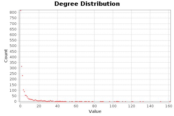
En cuanto a grados totales, hay cuatro nodos que destacan, con un grado de mayor a 120. El nodo con mayor grado es de 161. Estos nodos se corresponden con hubs. La distribución de grados indica que se cumple la propiedad libre de escala. Muy pocos con muchas conexiones, y muchos con pocas conexiones.
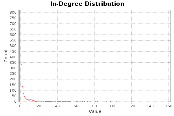
Los nodos con mayor grado de entrada (Con mayor número de seguidores) tienen 120 y 160 seguidores, respectivamente.
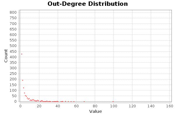
Pasa absolutamente lo mismo para los grados de entrada y salida, en el caso de Twitter esto indica seguidores y seguidos. El usuario con más amigos tiene unos 99 amigos.
Diámetro
El diámetro de la red es de 13. Este valor representa la máxima distancia existente entre dos nodos en toda la red. La distancia media es de 4.5.
El histograma de distancias es el siguiente:
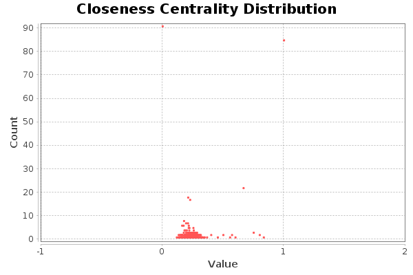
El diagrama de cercanía nos indica que hay bastantes nodos muy alejados del centro (entorno a unos 90). Otros, por contra, están muy situados en el centro de la red (unos 85). El resto de nodos se situan a los alrededores del centro de la red.
Conectividad
Se tienen 845 componentes conexas, la componente gigante agrupa 1261 nodos. El coeficiente de clustering medio es 0.068. En este caso es bajo, ya que la cuenta de twitter es de un blog, en lugar de una cuenta personal. El histograma CC es el siguiente:

Lo cual indica que en regiones poco pobladas el coeficiente de clustering es muy alto, ya que los nodos están más conectados entre ellos localmente. Por ello destaca un punto muy alto al principio de la gráfica.
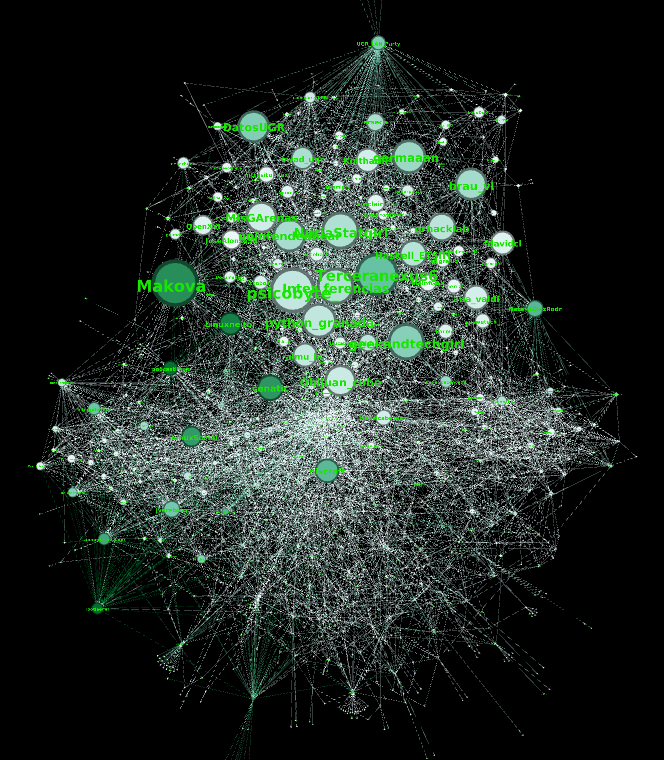
Centralidad de los actores
Los cinco primeros actores para las siguientes medidas son:
| Centralidad de Grado | Intermediación | Cercanía | Vector propio |
|---|---|---|---|
| nixcraft: 161 | rootjaeger: 0.048 | programador4web: 1 | Makova_: 1 |
| Makova_: 151 | podcastlinux: 0.048 | KevinhoMorales: 1 | psicobyte_: 0.966 |
| cenatic: 132 | Linuxneitor: 0.043 | elrne: 1 | Terceranexus6: 0.908 |
| Terceranexus6: 129 | Makova_: 0.039 | Mrcoo16: 1 | NuriaStatgirl: 0.796 |
| LignuxSocial: 121 | Wdesarrollador: 0.038 | RodriKing14: 1 | Inter_ferencias: 0.780 |
En cuanto a la centralidad de grado, no se tiene muy en cuenta, aunque refleja el número de conexiones de un actor, no tiene en cuenta la estructura global de la red.
Una medida bastante importante es la intermediación, estos actores hacen de puente entre otras regiones de la red. Por lo cual pueden conectar distintas comunidades entre sí. En el caso que nos ocupa (Twitter), si conseguimos que uno de estos actores nos mencione o nos haga RT, nuestro tweet podrá llegar a otro tipo de usuarios que quizá estén interesados en nuestras ideas.
La cercanía mide cómo de cerca está un actor del centro de la red. En este caso no nos sirve de mucho, ya que todos los nodos tienen la misma medida.
Por último, la centralidad de vector propio es una medida recursiva que asigna importancia a un nodo en función de la importancia de sus vecinos. Es decir, tiene en cuenta la calidad de las conexiones, en lugar de la cantidad. El primer actor tiene un valor de esta medida de 1, lo cual indica que es el nodo más importante y con el mayor número de conexiones importantes. Luego es un actor a tener en cuenta en la red.
Detección de comunidades
Para la detección de comunidades se ha usado un factor de resolución de 1.99 para obtener un total de 5 comunidades. Se ha elegido este valor de resolución debido a que valores inferiores resultaban en un mayor número de comunidades, pero muchas de ellas formadas por dos nodos. El valor para la modularidad es de un 0.436, lo cual es un buen valor.
La proporción de nodos en cada comunidad es la siguiente:
- 40.85%
- 21.39%
- 17.5%
- 10.98%
- 9.15%
- 0.14%
La distribución de modularidad se observa en la siguiente imagen:

Todas tienen un tamaño razonable salvo una, demasiado pequeña.
La siguiente imagen muestra el grafo coloreado en función de a qué comunidad pertenece cada nodo:
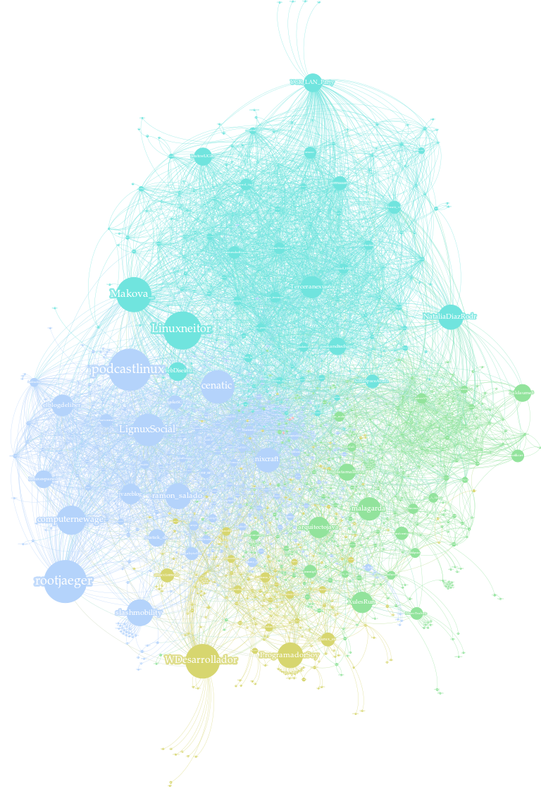
Analizando la red, se puede apreciar que la comunidad de arriba (Azul celeste) pertenece a nodos relacionados con la ETSIIT. Algunos miembros de esta comunidad hacen de puente (Son nodos con mucha intermediación) con otras comunidades. Por ejemplo, Makova_ y Linuxneitor hacen de puente con la comunidad morada, esta comunidad está más relacionada con usuarios de Linux y blogs de Linux. NataliaDiazRodrz hace de puente de la comunidad de la ETSIIT con la comunidad verde, más relacionada con la temática de Ciencia de Datos. Esto tiene sentido, ya que NataliaDiazRodrz estudió en la ETSIIT y trabaja en Ciencia de Datos, concretamente en temas de NLP. La comunidad Amarilla está relacionada con programación.
Gráficos adicionales
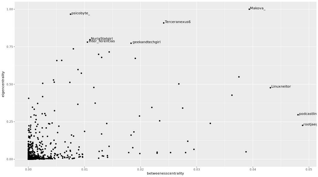
En la siguiente gráfica se muestra la red dispuesta con los colores en función del valor del vector propio, y el tamaño de los nodos como la intermediación:

En la siguiente figura se muestra a la inversa, color la intermediación, tamaño el vector propio:
Considero que las medidas más importantes son el valor de vector propio y la intermediación, la siguiente gráfica muestra cómo están relacionadas entre ellas. A mayor valor para ambas mejor, más importante es el nodo:
DONE An analysis and visualization of my twitter account with Gephi
This article is the result of an exercise for the subject Mining of Social Media in the Master’s Degree in Data Science at the UGR
Network analysis
This network contains a subset of the followers of the Twitter account @elbaulp, since due to API limitations the download of the network up to the second degree of connection took a long time.
The objective of this analysis is to identify the most influential actors, who act as a bridge between communities in order to expand the number of followers of @ElbaulP.
Average degree
- N = 2132 nodes.
- L = 6643 links
- Density = 0.001
- Average grade = 3.116, which means that each node of the network is connected to another 3 on average.
The density graphs of the degrees are shown below.
In terms of total grades, there are four nodes that stand out, with a grade greater than 120. The node with the highest grade is 161. These nodes correspond to hubs. The distribution of degrees indicates that the property is fulfilled free of scale. Very few with many connections, and many with few connections.
The nodes with the highest degree of input (with the highest number of followers) have 120 and 160 followers, respectively.
It is absolutely the same for the degrees of entry and exit, in the case of Twitter this indicates followers and followers. The user with more friends has about 99 friends.
Diameter
The diameter of the network is 13. This value represents the maximum distance between two nodes in the entire network. The average distance is 4.5.
The distance histogram is as follows:
The closeness diagram shows that there are quite a few nodes very far from the centre (around 90). Others, on the other hand, are very located in the centre of the network (about 85). The rest of the nodes are located around the centre of the network.
Connectivity
There are 845 related components, the giant component groups 1261 nodes. The average clustering coefficient is 0.068. In this case it is low, since the twitter account is a blog account, rather than a personal account. The CC histogram is as follows:
This indicates that in sparsely populated regions the clustering coefficient is very high, as the nodes are more locally connected to each other. For this reason, a very high point stands out at the beginning of the graph.
Betweeness Centrality
The first five actors for the following measures are:
| Centralidad de Grado | Intermediación | Cercanía | Vector propio |
|---|---|---|---|
| nixcraft: 161 | rootjaeger: 0.048 | programador4web: 1 | Makova_: 1 |
| Makova_: 151 | podcastlinux: 0.048 | KevinhoMorales: 1 | psicobyte_: 0.966 |
| cenatic: 132 | Linuxneitor: 0.043 | elrne: 1 | Terceranexus6: 0.908 |
| Terceranexus6: 129 | Makova_: 0.039 | Mrcoo16: 1 | NuriaStatgirl: 0.796 |
| LignuxSocial: 121 | Wdesarrollador: 0.038 | RodriKing14: 1 | Inter_ferencias: 0.780 |
As for the grade centrality, it is not very much taken into account, although it reflects the number of connections of an actor, it does not take into account the overall structure of the network.
An important measure is intermediation, these actors act as a bridge between other regions of the network. So they can connect different communities to each other. In the case at hand (Twitter), if we get one of these actors to mention us or do RT, our tweet could reach other types of users who might be interested in our ideas.
The closeness measures how close an actor is to the center of the network. In this case it doesn’t help us much, since all the nodes have the same measure.
Finally, the own vector core is a recursive measure that assigns importance to a node according to the importance of its neighbors. That is, it takes into account the quality of connections, rather than quantity. The first actor has a value of this measure of 1, which indicates that it is the most important node and with the greatest number of important connections. It is then an actor to be taken into account in the network.
Community detection
For the detection of communities, a resolution factor of 1.99 has been used to obtain a total of 5 communities. This resolution value was chosen because lower values resulted in a greater number of communities, but many of them formed by two nodes. The value for modularity is 0.436, which is a good value.
The proportion of nodes in each community is as follows:
- 40.85%
- 21.39%
- 17.5%
- 10.98%
- 9.15%
- 0.14%
The modularity distribution can be seen in the following image:
All are reasonably sized except one, which is too small.
The following image shows the colored graph according to which community belongs to each node:
Analyzing the network, it can be seen that the community above (sky blue) belongs to nodes related to ETSIIT. Some members of this community act as a bridge (they are nodes with a lot of intermediation) with other communities. For example, Makova_ and Linuxneitor bridge with the purple community, this community is more related to Linux users and Linux blogs. NataliaDiazRodrz bridges the ETSIIT community with the green community, more related to the Data Science theme. This makes sense, since NataliaDiazRodrz studied at ETSIIT and works in Data Science, specifically in NLP topics. The Amarilla community is related to programming.
Additional plots
The following graph shows the network arranged with the colors according to the value of the vector itself, and the size of the nodes as the intermediation:
In the following figure the inverse is shown, color the intermediation, size the own vector:
I consider that the most important measures are the own vector value and the intermediation, the following graphic shows how they are related between them. The higher the value for both the better, the more important the node:
¿Has visto algún error?: Por favor, ayúdame a corregirlo contactando conmigo o comentando abajo.